Chapter 2 Rarefaction Practice in Microbiome Data Analysis

Presented at the DataScience Group meeting, Quadram Institute Bioscience, July 2023

Co-author of this chapter: Andrea Telatin²

In the last decade, there has been ongoing debate regarding the optimal approach for normalizing sequencing depth in samples analyzed using 16S rRNA gene sequencing. A highly influential paper by McMurdie and Holmes (McMurdie and Holmes, 2014) strongly argued against the practice of rarefying sequence counts, deeming it “inadmissible” and discouraging its utilization. Despite a rebuttal on this subject (Weiss et al., 2017), which demonstrated the benefits of rarefying in certain cases, the proponents of alternative normalization method seem to have a predominant influence within the microbiome research community. Nevertheless, a recent publication by Patrick Schloss (Schloss, 2023), shows that rarefaction is the most robust approach to control for uneven sequencing effort when considered across a variety of alpha and beta diversity metrics.

2.1 Aims of this chapter

Collect some definitions and clarify the difference between the terms “rarefy” and “rarefaction”;
exemplify the previous terms in alpha and beta diversity analyses;
provide the code to implement rarefaction curves and to estimate rarefaction estimates of richness and Bray-Curtis dissimilarities.

2.2 Required packages

List of libraries used:

mia (BiocManager::install("mia"))
miaViz (BiocManager::install("miaViz"))
ape (install.packages("ape"))
scater (BiocManager::install("scater"))
patchwork (install.packages('patchwork'))
ranacapa (devtools::install_github("gauravsk/ranacapa"))
BiocParallel (BiocManager::install("BiocParallel"))
TreeSummarizedExperiment (BiocManager::install("TreeSummarizedExperiment"))

To install ranacapa you will need devtools (package) and phyloseq from bioconductor.

2.3 Introduction and definitions

Rarefaction in microbiome research was introduced from ecology research out of the need to address the issue of uneven sampling depth. When studying microbial communities using high-throughput sequencing techniques like 16S rRNA gene sequencing or shotgun metagenomics, the number of sequencing reads obtained from different samples can vary significantly. This uneven sampling depth can introduce biases and make it challenging to compare the diversity and abundance of microbial taxa between samples accurately.

Rarefaction standardises the sampling effort across all samples and should ensure fair comparisons of diversity and abundance. By repeatedly subsampling the sequencing data to a common sequencing depth for each sample, the rarefaction method allows researchers to obtain a consistent and unbiased estimate of the microbial diversity present in each sample.

Library size normalization by random subsampling without replacement is called rarefying. There is confusion in the literature regarding terminology, and sometimes this normalization approach is conflated with a non-parametric resampling technique, called rarefaction. According to (McMurdie and Holmes, 2014), rarefying is most often defined by the following steps:

Select a minimum library size, \(N_{L,min}\). This has also been called the rarefaction level.
Discard libraries (microbiome samples) that have fewer reads than \(N_{L,min}\).
Subsample the remaining libraries without replacement such that they all have size \(N_{L,min}\).

Let’s make a practical example in R. We start by creating a very simple count matrix with 3 taxa and 2 samples.

# Generate a very simple count matrix where the first
# sample has half the library size of the second sample
count_matrix <- matrix(c(68, 32, 200, 200, 200, 200), 
    nrow = 3, ncol = 2)
colnames(count_matrix) <- c("S1", "S2")
rownames(count_matrix) <- c("Taxa1", "Taxa2", "Taxa3")

count_matrix

##        S1  S2
## Taxa1  68 200
## Taxa2  32 200
## Taxa3 200 200

S2 sample has a library size which is twice the library size of sample S1.

colSums(count_matrix)

##  S1  S2 
## 300 600

According to the definition, we choose \(N_{L,min} = 300\) and we subsample, without replacement (random number generation seed equal to 123, see why), the counts such that they all the samples have size \(300\).

# Function to rarefy counts of a count matrix
rarefy_function <- function(count_matrix) {
  
  # Determine the minimum library size across samples
  minLibSize <- min(colSums(count_matrix))
  
  # Perform rarefaction on each sample in the count matrix
  count_rarefy <- apply(count_matrix, 2, FUN = function(smpl){
    
      # Create a vector of taxon names proportional to their counts in the sample
      vec <- rep(rownames(count_matrix), times = smpl)
        
      # Perform subsampling by randomly selecting taxon names without replacement
      subsampling <- sample(vec, size = minLibSize, replace = FALSE)
        
      # Create a table of the subsampled taxon counts
      table(subsampling)
  })
  
  return(count_rarefy)
}

# Set the random seed for reproducibility 
set.seed(123)

rarefied_counts <- rarefy_function(count_matrix)
rarefied_counts

##        S1  S2
## Taxa1  68 103
## Taxa2  32 109
## Taxa3 200  88

The resulting table is a table where the S1 remains the same as before subsampling. Indeed, subsampling \(N_{L,min} = 300\) counts from a sample with that same library size is like taking the entire sample. S2 instead, has now a total of 300 counts divided across the three taxa.

As the subsampling step is performed only once, another way to obtain the rarefied counts more easily, is to divide the counts by their library size, multiply the relative abundances by \(N_{L,min} = 300\), and round the results.

rarefy_simple_function <- function(count_matrix) {
  
  # Determine the minimum library size across samples
  minLibSize <- min(colSums(count_matrix))
  
  # Perform simple rarefaction on each sample in the count matrix
  count_rarefy_simple <- apply(count_matrix, 2, FUN = function(smpl){
    
    # Calculate the relative abundance of each taxon in the sample
    rel_abundance <- smpl / sum(smpl)
    
    # Multiply the relative abundances by Lmin to obtain the rarefied counts
    rarefied_counts <- round(minLibSize * rel_abundance, digits = 0)
    
    # Return the rarefied counts for the current sample
    return(rarefied_counts)
  })
  
  return(count_rarefy_simple)
}
count_rarefied_simple <- rarefy_simple_function(count_matrix)
count_rarefied_simple

##        S1  S2
## Taxa1  68 100
## Taxa2  32 100
## Taxa3 200 100

According to (Schloss, 2023), the authors of (McMurdie and Holmes, 2014) were correct to state that the distinction between “rarefying” and “rarefaction” was confusing and led to their conflation. However, they poorly managed to solve the problem due to misleading sentences throughout the publication. Traditionally, repeating the subsampling step a large number of times and averaging the result is called rarefaction. Instead, rarefying or subsampling is rarefaction, but with a single randomization. To minimize confusion, we will use “subsampling” in place of “rarefying” through the rest of this chapter. For clarity, we will use the same definition of rarefaction of (Schloss, 2023):

Select a minimum library size, \(N_{L,min}\). Researchers are encouraged to report the value of \(N_{L,min}\).
Discard samples that have fewer reads than \(N_{L,min}\).
Subsample the remaining libraries without replacement such that they all have size \(N_{L,min}\).
Compute the desired metric (e.g., richness, Shannon diversity, Bray-Curtis distances) using the subsampled data.
Repeat steps 3 and 4 a large number of iterations (typically 100 or 1,000). Researchers are encouraged to report the number of iterations.
Compute summary statistics (e.g., the mean) using the values from step 4.

2.4 Rarefaction in practice

The rarefaction, i.e. repeating the subsampling step a large number of times and averaging the result, is here exemplified for Richness index and Bray-Curtis dissimilarity index.

Let’s start by using an example dataset from a research published in PNAS in early 2011 (Caporaso et al., 2011). This work compared the microbial communities from 25 environmental samples and three known “mock communities” – a total of 9 sample types – at a depth averaging 3.1 million reads per sample. The dataset comes with the mia package.

library(mia)
data("GlobalPatterns", package = "mia")

# See https://microbiome.github.io/mia/reference/agglomerate-methods.html
gp_genus <- mia::agglomerateByRank(GlobalPatterns, "Genus")

# Filter out rows (taxa) with zero counts across all samples
gp_genus <- gp_genus[
    rowSums(assay(gp_genus, "counts")) > 0, ]

library(scater)
gp_genus <- addPerCellQC(gp_genus)

Here we show the distribution of library sizes across samples. We have library sizes ranging from 58688 reads to 40x times more.

library(miaViz)
summary(colData(gp_genus)$sum)

##    Min. 1st Qu.  Median    Mean 3rd Qu.    Max. 
##   58688  567103 1106849 1085257 1527330 2357181

# Create a scatter plot of the 'gp_genus' dataset, where the y-axis represents the 'sum' column in the colData,
# the x-axis represents the 'SampleType' column in the colData, and the points are colored by the 'SampleType' column
plotColData(object = gp_genus, 
    y = "sum", x = "SampleType", 
    colour_by = "SampleType") + 
    theme(axis.text.x = element_text(angle = 45, hjust=1))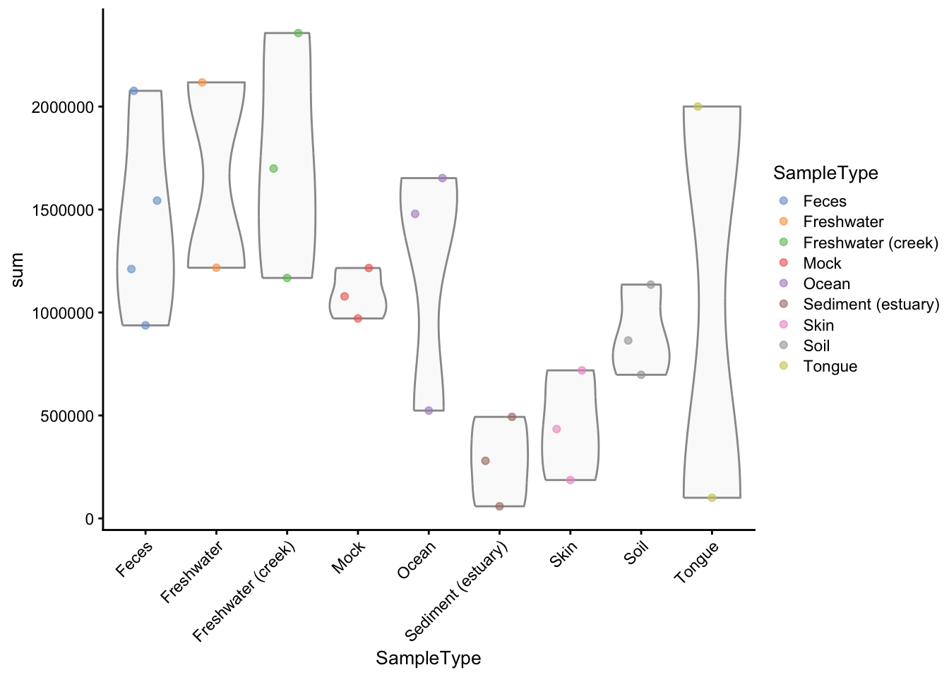

Figure 2.1: Sample library sizes grouped and coloured by sample type.

2.4.1 Richness index

Richness refers to the overall count of species within a community (sample). The most basic richness index corresponds to the number of observed species (observed richness). Richness estimates remain unaffected by the abundances of individual species.

To compute richness we use the estimateRichness function of the mia package.

gp_genus <- mia::estimateRichness(gp_genus, 
    assay.type = "counts", 
    index = "observed")

We can inspect the observed richness distribution of each sample type:

p_r <- plotColData(object = gp_genus, 
    y = "observed", x = "SampleType", 
    colour_by = "SampleType") + 
    theme(axis.text.x = element_text(angle = 45, hjust=1)) + 
    labs(title = "Richness in raw counts")
p_r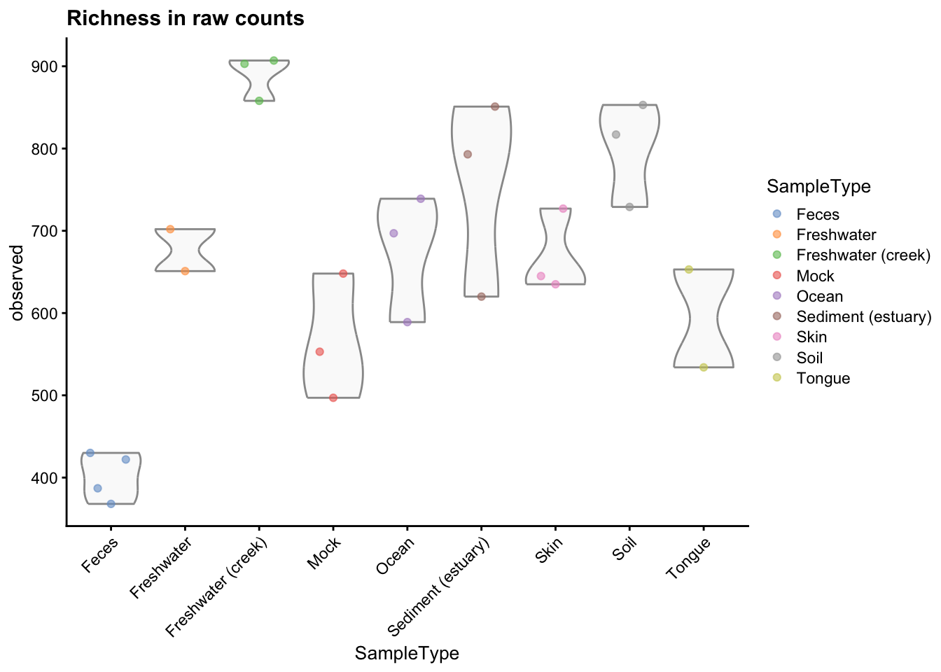

Figure 2.2: Richness estimates grouped and coloured by sample type.

And we can also describe the relationship between library size and richness. When the sequencing depth is enough to describe the samples we do not expect to see any particular pattern in this kind of graphical representation.

plotColData(object = gp_genus, 
    x = "sum", y = "observed", 
    colour_by = "SampleType") + 
    geom_smooth() + 
    labs(x = "Library Size", y = "Richness", 
         title = "Richness vs Library Size")

## `geom_smooth()` using method = 'loess' and
## formula = 'y ~ x'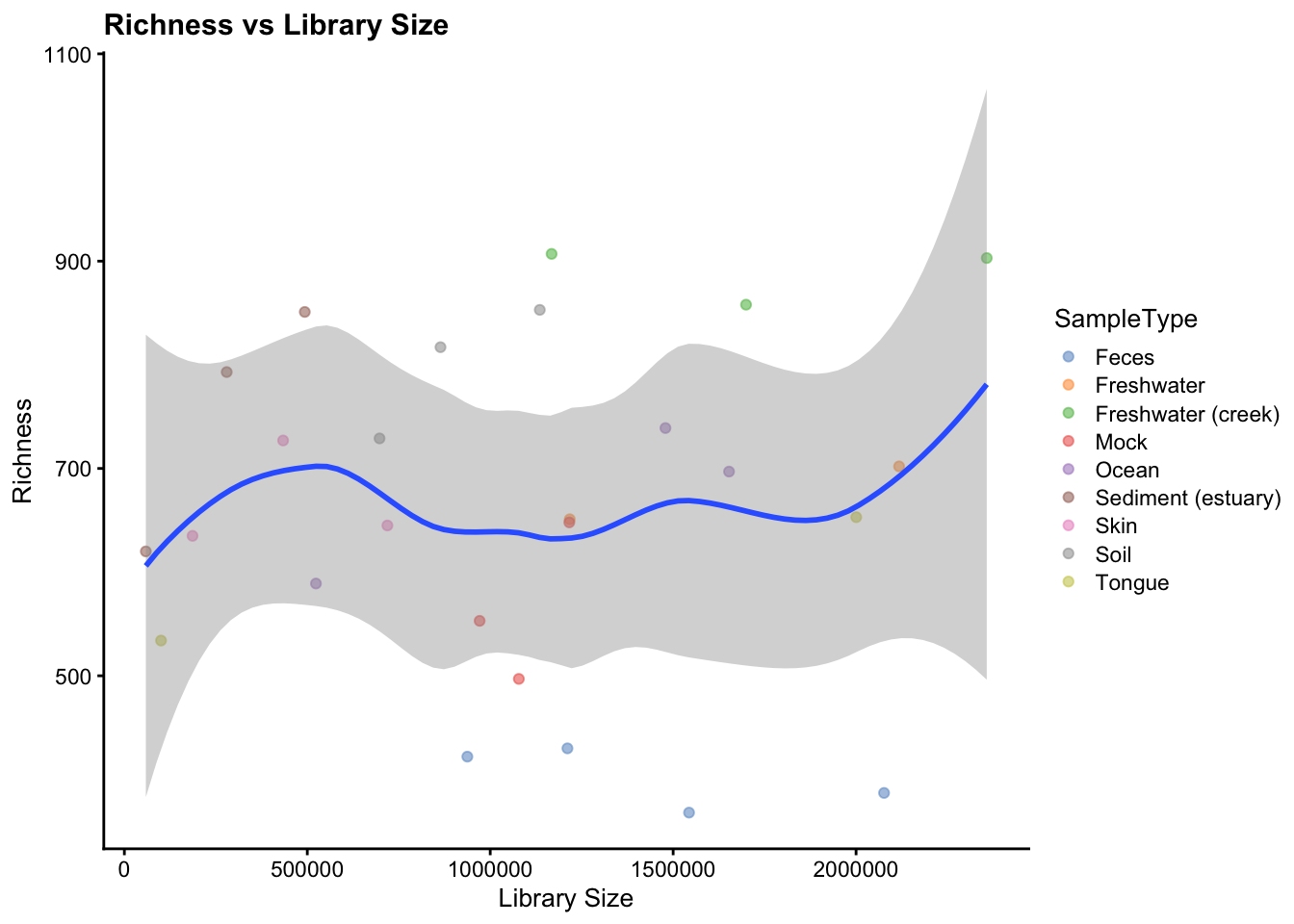

Figure 2.3: Relationship between richness and library size coloured by sample type.

But all of the above plots are generated from raw data. Here we want to inspect the effect of rarefaction. For this reason we use the subsampleCounts function of the package mia to obtain subsampled counts. We repeat this process 3 times with 3 different seeds (1, 2, and 3). We store the results in three differentially named assays of the TreeSummarizedExperiment object: rare1, rare2, and rare3.

gp_genus <- mia::subsampleCounts(gp_genus, 
    assay.type = "counts", 
    min_size = min(gp_genus$sum), 
    seed = 1, replace = FALSE, 
    verbose = FALSE, 
    name = "rare1")
gp_genus <- mia::subsampleCounts(gp_genus, 
    assay.type = "counts", 
    min_size = min(gp_genus$sum), 
    seed = 2, replace = FALSE, 
    verbose = FALSE, 
    name = "rare2")
gp_genus <- mia::subsampleCounts(gp_genus, 
    assay.type = "counts", 
    min_size = min(gp_genus$sum), 
    seed = 3, replace = FALSE, 
    verbose = FALSE, 
    name = "rare3")

We compute richness for each subsampled count matrix:

gp_genus <- estimateRichness(gp_genus, assay.type = "rare1", name = "rich1", index = "observed")
gp_genus <- estimateRichness(gp_genus, assay.type = "rare2", name = "rich2", index = "observed")
gp_genus <- estimateRichness(gp_genus, assay.type = "rare3", name = "rich3", index = "observed")

And plot the results:

p_r1 <- plotColData(object = gp_genus, 
    y = "rich1", x = "SampleType", 
    colour_by = "SampleType") + 
    theme(axis.text.x = element_text(angle = 45, hjust=1)) + 
    labs(title = "Subsampled counts - seed = 1", 
         subtitle = paste("N(L,min) =", min(gp_genus$sum)))
p_r2 <- plotColData(object = gp_genus, 
    y = "rich2", x = "SampleType", 
    colour_by = "SampleType") + 
    theme(axis.text.x = element_text(angle = 45, hjust=1)) + 
    labs(title = "Subsampled counts - seed = 2", 
         subtitle = paste("N(L,min) =", min(gp_genus$sum)))
p_r3 <- plotColData(object = gp_genus, 
    y = "rich3", x = "SampleType", 
    colour_by = "SampleType") + 
    theme(axis.text.x = element_text(angle = 45, hjust=1)) + 
    labs(title = "Subsampled counts - seed = 3", 
         subtitle = paste("N(L,min) =", min(gp_genus$sum)))

library(patchwork)
(plot_spacer() + p_r + plot_spacer()) / (p_r1 + p_r2 + p_r3) + 
    plot_layout(guides = "collect") + plot_annotation(tag_levels = "a")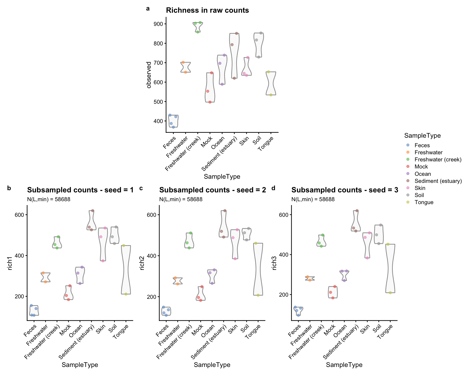

Richness estimates grouped and coloured by sample type. a) Raw data. b) subsampled counts, seed = 1. c) subsampled counts, seed = 2. d) subsampled counts, seed = 3.

Figure 2.4: Richness estimates grouped and coloured by sample type. a) Raw data. b) subsampled counts, seed = 1. c) subsampled counts, seed = 2. d) subsampled counts, seed = 3.

The main difference in these panels are the range of the y-axis: it reaches higher values in a rather than b, c, and d. Moreover, while the richest samples belonged to Freshwater (creek) when the richness was evaluated using raw counts (panel a), Sediment (estuary) samples became the richest when the subsampled counts were used instead (b, c, and d panels). This is probably due to the differential presence of rare taxa between the two environments. Minor differences are observable when comparing b, c, and d panels, but still, they are present.

Practically, rarefaction consists in averaging the index measures of panels b, c, and d to obtain a single value for each sample.

gp_genus$rich_rarefaction <- rowMeans(
    as.data.frame(colData(gp_genus)[, 
        c("rich1", "rich2", "rich3")]))
p_rarefaction <- plotColData(object = gp_genus, 
    y = "rich_rarefaction", x = "SampleType", 
    colour_by = "SampleType") + 
    theme(axis.text.x = element_text(angle = 45, hjust=1)) + 
    labs(title = "Rarefaction Richness", 
         subtitle = paste("Subsamplings = 3, N(L,min) =", 
            min(gp_genus$sum)))
p_rarefaction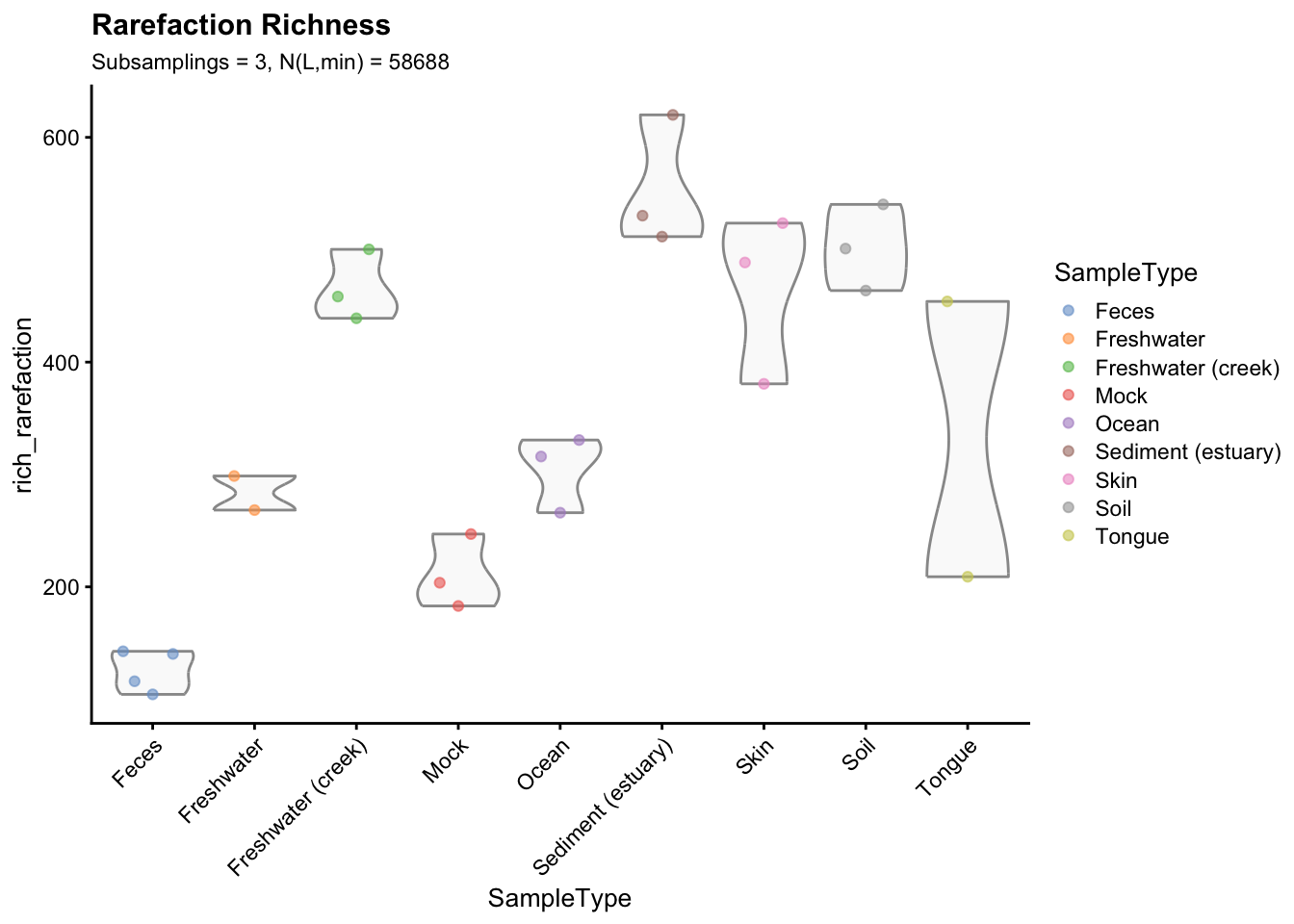

Richness estimates grouped and coloured by sample type. Richness indexes were averaged across the 3 subsamplings to obtain a single value for each sample.

Figure 2.5: Richness estimates grouped and coloured by sample type. Richness indexes were averaged across the 3 subsamplings to obtain a single value for each sample.

To automatise the entire procedure the following function can be used:

library(BiocParallel)

rarefaction_richness <- function(
    tse, # The object to use
    assay.type = "counts", # Assay to use
    subsamplings = 100, # Number of subsamplings
    minLibSize = NULL, # The desired library size 
    seed = 123, # The seed
    BPPARAM = SerialParam()){ # Parallelisation
    
    counts <- assay(tse, "counts")
    
    if(is.null(minLibSize))
        minLibSize <- min(colSums(counts))
    
    richness_list <- bplapply(
        X = 1:subsamplings, 
        BPPARAM = BPPARAM, 
        BPOPTIONS = bpoptions(RNGseed = seed), 
        FUN = function(sub){
            # Subsampling step
            tse <- mia::subsampleCounts(tse, 
                assay.type = assay.type, 
                min_size = minLibSize,
                # seed = runif(1, 0, .Machine$integer.max), 
                replace = FALSE, 
                verbose = FALSE, 
                name = "sub")
            # Estimation step
            richness <- mia::estimateRichness(tse, 
                assay.type = "sub", 
                index = "observed", 
                name = "richness")$richness
            return(richness)
    })
    # Return the averaged values
    colMeans(plyr::ldply(richness_list))
}

We run it in parallel (Linux or MacOS, Windows users should use BPPARAM = SerialParam()) and we directly store the computed values inside the TreeSummarizedExperiment object.

library("TreeSummarizedExperiment")
gp_genus$rarefaction_richness <- rarefaction_richness(
    tse = gp_genus, 
    assay.type = "counts", 
    subsamplings = 100, 
    BPPARAM = MulticoreParam(4), 
    minLibSize = NULL, 
    seed = 123)

Finally, the graphical representation of rarefied richness (seed = 123, number of subsamplings = 100, \(N_{L,min} = 58688\)) is reported below.

p_rarefaction100 <- plotColData(object = gp_genus, 
    y = "rarefaction_richness", x = "SampleType", 
    colour_by = "SampleType") + 
    theme(axis.text.x = element_text(angle = 45, hjust=1)) + 
    labs(title = "Rarefaction Richness", 
         subtitle = paste("Seed = 123, Subsamplings = 100, N(L,min) =", 
            min(gp_genus$sum)))
p_rarefaction100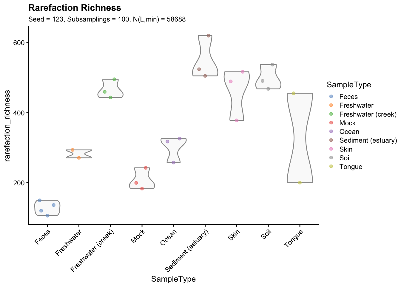

Richness estimates grouped and coloured by sample type. Richness indexes were averaged across 100 subsamplings (rarefaction library size = 58688) to obtain a single value for each sample (seed = 123).

Figure 2.6: Richness estimates grouped and coloured by sample type. Richness indexes were averaged across 100 subsamplings (rarefaction library size = 58688) to obtain a single value for each sample (seed = 123).

2.4.2 Rarefaction curves

One of the most informative application that involves rarefaction and microbial richness is the creation of rarefaction curves:

# devtools::install_github("gauravsk/ranacapa")
library(ranacapa)
set.seed(123)
rarefaction_curves <- ggrare(
    mia::makePhyloseqFromTreeSE(gp_genus), 
    step = 10000, plot = FALSE, parallel = TRUE)

library(ggplot2)
# https://rdrr.io/github/LTLA/scater/src/R/plot_colours.R
total_colors <- scater:::.get_palette("tableau10medium")[1:9]
names(total_colors) <- levels(gp_genus$SampleType)

print(rarefaction_curves) + 
    geom_line(aes(color = SampleType)) + 
    facet_wrap(~ SampleType, nrow = 3, ncol = 3) + 
    scale_color_manual(values = total_colors) +
    theme(axis.text.x = element_text(angle = 45, hjust = 1)) + 
    labs(title = "Rarefaction curves",
         subtitle = "Faceted by sample type")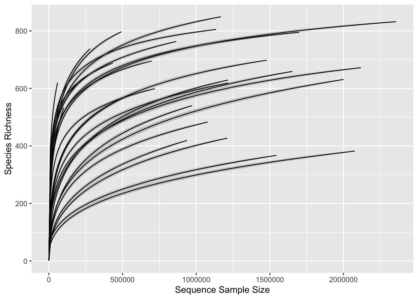

Figure 2.7: Rarefaction curves.

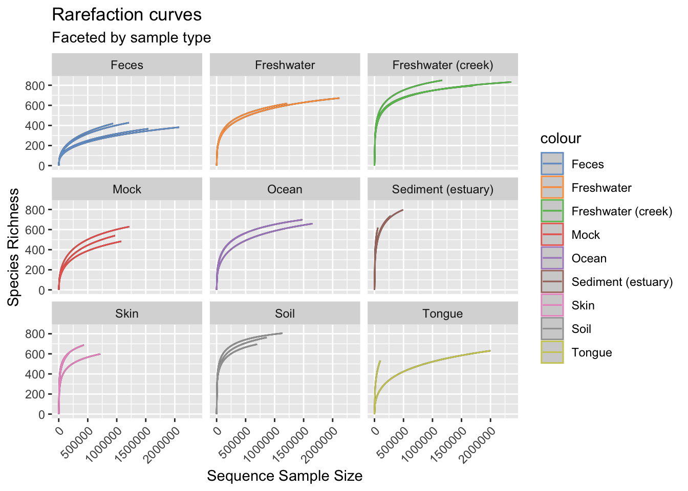
Figure 2.8: Rarefaction curves.

In this case the process of rarefaction consists in repeatedly subsampling the sequencing data at different depths, typically starting from the smallest number of reads in any sample to the largest. At each subsampling depth, the number of observed taxa is calculated (i.e., richness), and these values are plotted against the corresponding sequencing depth. The resulting curve shows how the diversity of the microbial community changes as the sequencing depth increases.

The importance of rarefaction curves lies in several key aspects:

Assessing data completeness. If the curves reach a plateau, it suggests that the sequencing depth is sufficient to capture most of the diversity in the sample. On the other hand, if the curves do not plateau (e.g., one tongue sample, and all Sediment (estuary) samples), it indicates that more sequencing effort is needed to adequately characterize the microbial diversity.
Fair comparison. Rarefaction curves enable fair comparisons of diversity across different samples with varying sequencing depths. By subsampling all samples to the same sequencing depth, the curves provide a standardized view of the community’s diversity, facilitating reliable comparisons.
Assessing quality. Rarefaction curves can help identify samples with low sequencing depth that might require additional attention or potentially be excluded from further analysis due to insufficient data.
Study design optimization. Researchers can use rarefaction curves during the study design phase to estimate the required sequencing depth for reliable and comprehensive community profiling. This information can help optimize cost-effectiveness and resource allocation.

2.4.3 Bray-Curtis dissimilarity index

Similarly to what we did for microbial richness, we can also study the effect of rarefaction on beta-diversity. In particular, we will focus on the Bray-Curtis dissimilarity index, a widely used metric to quantify the dissimilarity or similarity between two ecological samples, typically used in the context of community ecology and biodiversity studies.

Here we start by computing the Bray-Curtis indexes on raw counts, relative abundances (Total Sum Scaling normalization), and some subsamplings (the same used earlier for richness). Then use Multi Dimensional Scaling unsupervised ordination method is used to visualize the results.

gp_genus <- transformCounts(gp_genus, 
    assay.type = "counts", method = "relabundance")

gp_genus <- runMDS(gp_genus,
    FUN = vegan::vegdist,
    method = "bray",
    name = "PCoA_BC_raw",
    assay.type = "counts")

gp_genus <- runMDS(gp_genus,
    FUN = vegan::vegdist,
    method = "bray",
    name = "PCoA_BC_TSS",
    assay.type = "relabundance")

gp_genus <- runMDS(gp_genus,
    FUN = vegan::vegdist,
    method = "bray",
    name = "PCoA_BC1",
    assay.type = "rare1")

gp_genus <- runMDS(gp_genus,
    FUN = vegan::vegdist,
    method = "bray",
    name = "PCoA_BC2",
    assay.type = "rare2")

gp_genus <- runMDS(gp_genus,
    FUN = vegan::vegdist,
    method = "bray",
    name = "PCoA_BC3",
    assay.type = "rare3")

p_bc_raw <- plotReducedDim(gp_genus, "PCoA_BC_raw", 
    colour_by = "SampleType") + 
    labs(title = "Raw counts, Bray-Curtis, PCoA")
p_bc_tss <- plotReducedDim(gp_genus, "PCoA_BC_TSS", 
    colour_by = "SampleType") + 
    labs(title = "TSS, Bray-Curtis, PCoA")
p_bc_r1 <- plotReducedDim(gp_genus, "PCoA_BC1", 
    colour_by = "SampleType")  + 
    labs(title = "Subsampled seed = 1, Bray-Curtis, PCoA",
         subtitle = paste("N(L,min) =", min(gp_genus$sum)))
p_bc_r2 <- plotReducedDim(gp_genus, "PCoA_BC2", 
    colour_by = "SampleType") + 
    labs(title = "Subsampled seed = 2, Bray-Curtis, PCoA",
         subtitle = paste("N(L,min) =", min(gp_genus$sum)))
p_bc_r3 <- plotReducedDim(gp_genus, "PCoA_BC3", 
    colour_by = "SampleType") +
    scale_y_reverse()  + 
    labs(title = "Subsampled seed = 3, Bray-Curtis, PCoA",
         subtitle = paste("N(L,min) =", min(gp_genus$sum)))

(p_bc_raw + p_bc_tss + plot_spacer()) / 
    (p_bc_r1 + p_bc_r2 + p_bc_r3) + 
    plot_layout(guides = "collect") +
    plot_annotation(tag_levels = "a")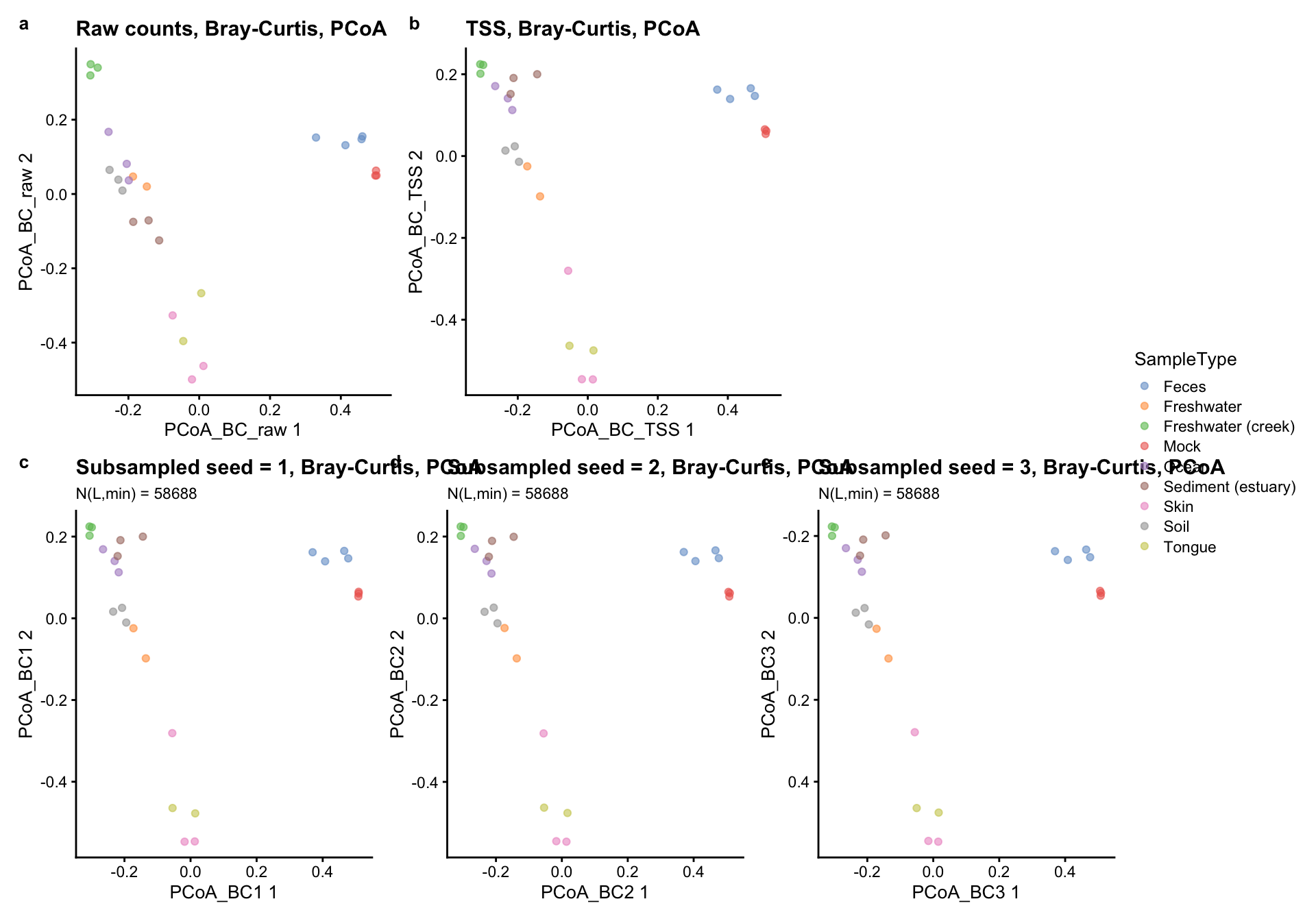

The main difference in these panels is only between a and all the others which are quite similar. That’s because in this case the total sum scaling normalization (panel b) behave similarly to using subsampling at the fixed library size of \(N_{L,min}=58688\) (panels c, d, and e).

The Bray-Curtis dissimilarity between two samples is computed following the formula:

\[ BC_{jk} = \frac{\sum_i|x_{ij}-x_{ik}|}{\sum_ix_{ij}+x_{ik}} \]

where \(i\) is the number of taxa and \(j,k\) are the sample indexes. By construction, when a sample has 10x more counts than the other, the numerator could be inflated just for this reason and not because of a real difference between the samples.

Practically, rarefaction consists in averaging the index measures of panels b, c, and d to obtain a single value for each sample.

# Recompute the distances
bc1 <- vegan::vegdist(x = t(assay(gp_genus, "rare1")), 
    method = "bray")
bc2 <- vegan::vegdist(x = t(assay(gp_genus, "rare2")), 
    method = "bray")
bc3 <- vegan::vegdist(x = t(assay(gp_genus, "rare3")), 
    method = "bray")

# Average the distances across subsamplings
bc_rarefaction <- (bc1 + bc2 + bc3) / 3

# Add the PCoA coordinates in a new reducedDim slot
# following the instructions in help("runMDS")
reducedDim(gp_genus, "PCoA_BCrarefaction") <- cmdscale(d = bc_rarefaction, k = 2, eig = TRUE)$points

plotReducedDim(gp_genus, "PCoA_BCrarefaction", 
    colour_by = "SampleType") + 
    labs(title = "Rarefaction Bray-Curtis, PCoA",
         subtitle = paste("subsamplings = 3, N(L,min) =", min(gp_genus$sum)))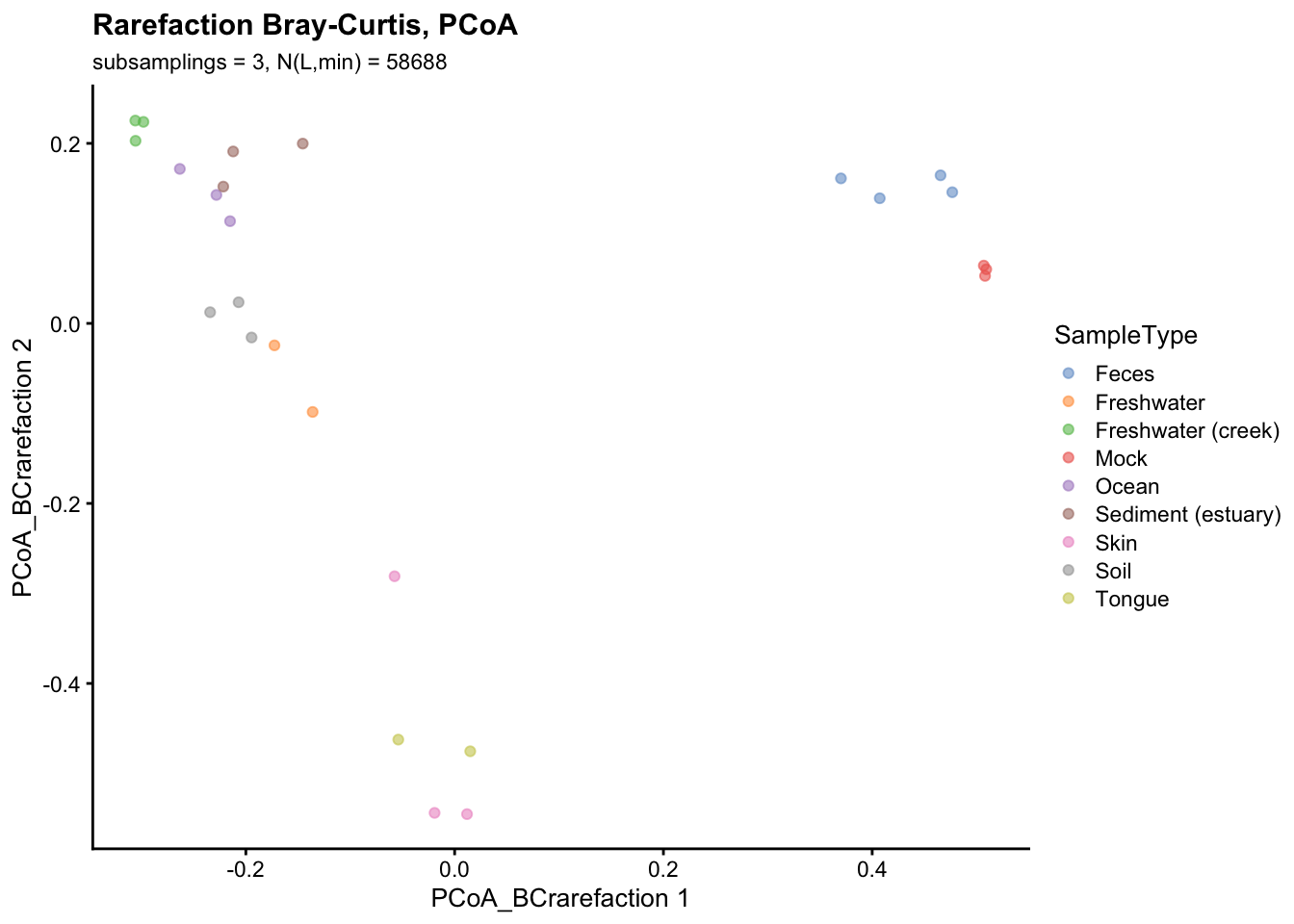

As we did for the richness index, the process can be automatised:

rarefaction_BC_PCoA <- function(
    tse, # The object to use
    assay.type = "counts", # Assay to use
    subsamplings = 10, # Number of subsamplings
    minLibSize = NULL, # The desired library size 
    seed = 123, # The seed
    BPPARAM = SerialParam()){ # Parallelisation
    
    counts <- assay(tse, "counts")
    
    if(is.null(minLibSize))
        minLibSize <- min(colSums(counts))
    
    dist_list <- bplapply(
        X = 1:subsamplings, 
        BPPARAM = BPPARAM, 
        BPOPTIONS = bpoptions(RNGseed = seed), 
        FUN = function(sub){
            # Subsampling step
            tse <- mia::subsampleCounts(tse, 
                assay.type = assay.type, 
                min_size = minLibSize,
                # seed = runif(1, 0, .Machine$integer.max), 
                replace = FALSE, 
                verbose = FALSE, 
                name = "sub")
            # BC calculation step
            BC_dist <- vegan::vegdist(
                x = t(assay(tse, "sub")),
                method = "bray")
            return(BC_dist)
    })
    # Compute the mean BC distance
    avg_BC_dist <- Reduce(f = '+', dist_list) / subsamplings
    # Compute the PCoA coordinates and return them
    cmdscale(d = avg_BC_dist, k = 2, eig = TRUE)$points
}

We run it in parallel (Linux or MacOS, Windows users should use BPPARAM = SerialParam()) and we directly store the computed values inside the TreeSummarizedExperiment object in the reducedDim slot.

reducedDim(gp_genus, "PCoA_BCrarefaction100") <- 
    rarefaction_BC_PCoA(
        tse = gp_genus, 
        assay.type = "counts", 
        subsamplings = 100,
        minLibSize = NULL, 
        seed = 321, 
        BPPARAM = MulticoreParam(4))

Finally, the graphical representation of rarefied beta-diversity using Bray-Curtis dissimilarity index and PCoA ordination (seed = 123, number of subsamplings = 100, \(N_{L,min} = 58688\)) is reported below.

plotReducedDim(gp_genus, "PCoA_BCrarefaction100", 
    colour_by = "SampleType") + 
    labs(title = "Rarefaction Bray-Curtis, PCoA",
         subtitle = paste("subsamplings = 100, seed = 321, N(L,min) =", min(gp_genus$sum))) + 
    scale_y_reverse()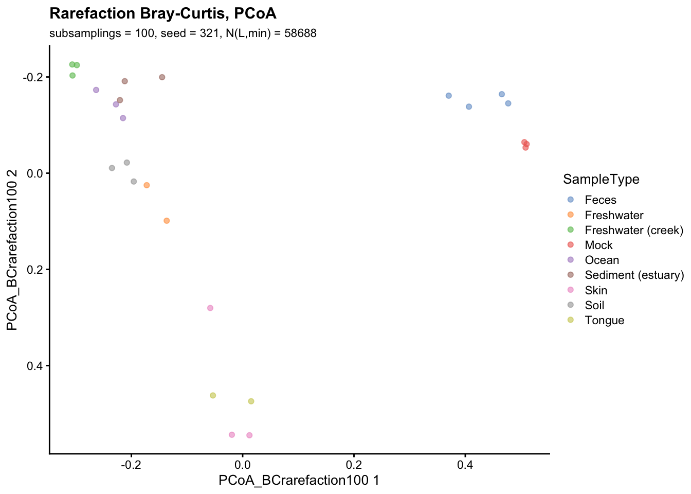

In this scenario rarefaction and Total Sum Scaling (TSS) normalization produced similar results. This is probably due to the fact that all samples are already at a sufficient depth to capture most of the microbial diversity.

But this can also occur when:

the differences in sequencing depth between samples are relatively small;
the samples have similar distributions of taxa and similar alpha diversity measures, so the impact of rarefaction or TSS normalization is minimal.

However, in cases where there are substantial differences in sequencing depth or if the samples have highly variable distributions of taxa, rarefaction and TSS normalization might lead to different results. In such situations, researchers should carefully consider which normalization approach is more appropriate for their specific dataset and research objectives.

2.5 Exercise: loading real datasets

To test R packages it’s convenient to rely on high-quality, polished datasets such as GlobalPatterns. In the real world, though, we need to load datasets produced by different packages (often in different formats), and to produce the appropriate data structures (e.g. a Phyloseq object) starting from our raw files.

In addition to a lot of data wrangling and format conversions, real data is noisy, contains errors or inconsistencies and we need to be able to perform some checks and eyeballing or we will miss the gorilla.

We have some files produced analysing the famous “MiSeq SOP” dataset from the laboratory of Pat Schloss himself (Schloss et al., 2012), based on a longitudinal study of gut microbiome stabilization in mice post-weaning.

The files analised here are available in the Github repository of this chapter:

dada2_stats.tsv: a summary of the performance of DADA2 denoising
feature-table.tsv: raw counts per feature (ASVs) per sample
metadata.tsv: properties of each sample
rep-seqs.tree: phylogenetic tree of the ASVs
taxonomy.txt: table with the taxonomic classification of each ASV

For the purpose of this chapter, we will not delve into the specific details on the reads to counts procedure, which will be discussed elsewhere soon.

2.5.1 Read the raw data

The pipeline used to identify the Amplicon Sequence Variants (ASV) is based on DADA2, and produced a table with some statistics on the procedure, called dada2_stats.tsv.

Ignoring similar tables can produce flawed analyses: sometimes only a very small fractions of reads passes all the filtering steps, so from a sequencing depth of 50.000 you can generate a counts table where the total is reduced to 1000. Such reduction must be addressed before doing any analysis.

# Read dada2 stats file
quality_stats <- read.delim("./data/01_rarefaction/dada2_stats.tsv", header = TRUE, sep = "\t")

# Add rownames
rownames(quality_stats) <- gsub(pattern = "_R1.fastq.gz", replacement = "", x = quality_stats[,"X"])

# Remove the first column
quality_stats <- quality_stats[, -1]

head(quality_stats)

##        input filtered denoised merged non.chimeric
## F3D0    7793     6302     6302   5636         5627
## F3D1    5869     4616     4616   4314         4304
## F3D141  5958     4897     4897   4221         4087
## F3D142  3183     2631     2631   2157         2113
## F3D143  3178     2624     2624   2193         2172
## F3D144  4827     3751     3751   3036         2882

Some kind of metadata file is usually part of the analysis, we have a minimal metadata file called metadata.tsv:

# Read metadata
metadata <- read.delim("./data/01_rarefaction/metadata.tsv", header = TRUE, sep = "\t", row.names = 1)

head(metadata)

##         Week                                                             Files
## F3D0   Early     F3D0_S188_L001_R1_001.fastq.gz,F3D0_S188_L001_R2_001.fastq.gz
## F3D1   Early     F3D1_S189_L001_R1_001.fastq.gz,F3D1_S189_L001_R2_001.fastq.gz
## F3D141  Late F3D141_S207_L001_R1_001.fastq.gz,F3D141_S207_L001_R2_001.fastq.gz
## F3D142  Late F3D142_S208_L001_R1_001.fastq.gz,F3D142_S208_L001_R2_001.fastq.gz
## F3D143  Late F3D143_S209_L001_R1_001.fastq.gz,F3D143_S209_L001_R2_001.fastq.gz
## F3D144  Late F3D144_S210_L001_R1_001.fastq.gz,F3D144_S210_L001_R2_001.fastq.gz

An algorithm has been used to assign the taxonomy to the identified representative sequences. The taxonomy table is called taxonomy.tsv.

# Read taxonomy
taxonomy <- read.delim("./data/01_rarefaction/taxonomy.txt", header = TRUE, sep = " ")
rownames(taxonomy) <- paste0("ASV", seq_len(nrow(taxonomy)))
head(taxonomy)

##       Kingdom       Phylum       Class         Order                     Family
## ASV1 Bacteria         <NA>        <NA>          <NA>                       <NA>
## ASV2     <NA>         <NA>        <NA>          <NA>                       <NA>
## ASV3 Bacteria Bacteroidota Bacteroidia Bacteroidales unclassified_Bacteroidales
## ASV4     <NA>         <NA>        <NA>          <NA>                       <NA>
## ASV5 Bacteria Bacteroidota Bacteroidia Bacteroidales             Bacteroidaceae
## ASV6     <NA>         <NA>        <NA>          <NA>                       <NA>
##            Genus
## ASV1        <NA>
## ASV2        <NA>
## ASV3        <NA>
## ASV4        <NA>
## ASV5 Bacteroides
## ASV6        <NA>

Finally, the central piece of information is the feature table (historically called “OTU Table”):

# Read feature table
feature_table <- read.delim("./data/01_rarefaction/feature-table.tsv", header = TRUE, sep = "\t", row.names = 1)
head(feature_table)

##      F3D0 F3D1 F3D141 F3D142 F3D143 F3D144 F3D145 F3D146 F3D147 F3D148 F3D149
## ASV1  556  377    422    279    216    387    609    311   1407    807    825
## ASV2  322  334    344    282    166    254    466    223   1127    676    735
## ASV3  416  210    319    149    185    281    472    233    860    548    676
## ASV4  402   64    455    155    221    325    539    376   1017    791    829
## ASV5  148  127    175    162    120     93    277    159    424    405    382
## ASV6  439   40    313    178    226    333    447    260   1091    818    599
##      F3D150 F3D2 F3D3 F3D5 F3D6 F3D7 F3D8 F3D9 Mock
## ASV1    298 3292  938  303  961  602  263  496    0
## ASV2    216 1486  560  256  643  488  333  403    0
## ASV3    381 1111  437  264  542  397  331  455    0
## ASV4    434  441  192  150  373  290  128  191    0
## ASV5    158  311  375  143  436  419  509  552    0
## ASV6    200  111   25   19   17    9    0    0    0

Sometimes it’s useful to know how related are the representative sequences, and this is usually done producing a multiple alignment from which a phylogenetic tree can be constructed.

An example of use of phylogenetic information is the computation of UniFrac distance.

# Read tree file
library(ape)
tree <- ape::read.tree(file = "./data/01_rarefaction/rep-seqs.tree")
str(tree)

## List of 5
##  $ edge       : int [1:443, 1:2] 224 225 226 227 228 229 230 230 229 231 ...
##  $ edge.length: num [1:443] 0.00906 0.00835 0.01424 0.00472 0.01043 ...
##  $ Nnode      : int 221
##  $ node.label : chr [1:221] "" "0.929" "0.764" "0.846" ...
##  $ tip.label  : chr [1:223] "ASV147" "ASV202" "ASV66" "ASV61" ...
##  - attr(*, "class")= chr "phylo"
##  - attr(*, "order")= chr "cladewise"

2.5.2 Assembling the `TreeSummarizedExperiment` object

tse <- TreeSummarizedExperiment(
    assays = list("counts" = feature_table),
    rowData = taxonomy, 
    colData = merge(metadata, quality_stats, by = 0),
    rowTree = tree)
tse

## class: TreeSummarizedExperiment 
## dim: 223 20 
## metadata(0):
## assays(1): counts
## rownames(223): ASV1 ASV2 ... ASV222 ASV223
## rowData names(6): Kingdom Phylum ... Family Genus
## colnames(20): F3D0 F3D1 ... F3D9 Mock
## colData names(8): Row.names Week ... merged non.chimeric
## reducedDimNames(0):
## mainExpName: NULL
## altExpNames(0):
## rowLinks: a LinkDataFrame (223 rows)
## rowTree: 1 phylo tree(s) (223 leaves)
## colLinks: NULL
## colTree: NULL

2.5.3 Compute quality metrics

For both the colData (i.e., sample metadata) and rowData (i.e., taxa metadata) slots of the experiment object we calculate some simple metrics. For the samples, the library size (sum) and the number of detected features (detected) are computed:

tse <- scater::addPerFeatureQC(tse)
tse <- scater::addPerCellQC(tse)

head(colData(tse)[, c("sum", "detected")])

## DataFrame with 6 rows and 2 columns
##              sum  detected
##        <numeric> <numeric>
## F3D0        5627       103
## F3D1        4304        94
## F3D141      4087        71
## F3D142      2113        49
## F3D143      2172        57
## F3D144      2882        45

For the taxa, their average count value (mean) and the percentage of samples with that feature (detected) are reported:

head(rowData(tse)[, c("mean", "detected")])

## DataFrame with 6 rows and 2 columns
##           mean  detected
##      <numeric> <numeric>
## ASV1    667.45        95
## ASV2    465.70        95
## ASV3    413.35        95
## ASV4    368.65        95
## ASV5    268.75        95
## ASV6    256.25        85

2.5.4 Filter or not to filter, this is the question

When we loaded the raw data, we may have noticed that many taxa were not classified, even at the kingdom and phylum level. In particular we have 20 ASVs which are not classified at the Kingdom level and 30 (the previous 20 plus other 10) at the Phylum level.

table(rowData(tse)$Kingdom, useNA = "always")

## 
## Bacteria     <NA> 
##      203       20

table(rowData(tse)$Phylum, useNA = "always")

## 
##      Actinobacteriota          Bacteroidota      Campilobacterota 
##                     6                     5                     1 
##         Cyanobacteria          Deinococcota            Firmicutes 
##                     3                     1                   166 
##       Patescibacteria        Proteobacteria unclassified_Bacteria 
##                     2                     7                     1 
##     Verrucomicrobiota                  <NA> 
##                     1                    30

Whether or not to remove unclassified features at the phylum level prior to every analysis in microbiome data depends on the specific goals and requirements of the analysis.

The presence of unclassified features may be due to various reasons, such as limited reference databases or low sequencing depth. On one hand, removing these unclassified features could improve data quality and reduce potential noise in your analysis. On the other hand, The decision to remove unclassified features may affect the outcome of the analysis. If the unclassified features are prevalent and significant in your dataset, removing them could lead to a loss of valuable information. Nevertheless, if they are rare or not biologically relevant, removing them might have minimal impact.

unclassified <- which(is.na(rowData(tse)$Phylum))
rowData(tse)[unclassified, c("mean", "detected")]

## DataFrame with 30 rows and 2 columns
##             mean  detected
##        <numeric> <numeric>
## ASV1      667.45        95
## ASV2      465.70        95
## ASV4      368.65        95
## ASV6      256.25        85
## ASV7      254.85        95
## ...          ...       ...
## ASV193      0.55         5
## ASV195      0.50        20
## ASV196      0.50         5
## ASV201      0.40         5
## ASV204      0.30        10

In our case we can see that some of the unclassified features are in the top abundant positions. These are hardly related to rare features as they are present with high mean abundances in more than 90% of the samples.

Whatever the choice, if you plan to share your data or replicate the analysis in the future, it’s essential to document clearly whether unclassified features were removed and the reasoning behind the decision.

2.5.5 Try again?

A closer inspection of the data raised an issue: multiple features (ASVs) had no taxonomy attached.

We noticed that high abundance and high prevalence features were not immune from the issue. If we can be sure that our taxonomy assignment was flawless, we might conclude we are observing new sequences, and it would be advisable to perform the analysis at the feature level, ignoring taxonomic lables when possible.

An alternative is to check our methods, and redo the taxonomy classification. Try loading taxonomy-dada.txt and you will now see a different story…

Bibliography

Caporaso,J.G. et al. (2011) Global patterns of 16S rRNA diversity at a depth of millions of sequences per sample. Proceedings of the National Academy of Sciences, 108, 4516–4522.

McMurdie,P.J. and Holmes,S. (2014) Waste Not, Want Not: Why Rarefying Microbiome Data Is Inadmissible. PLOS Computational Biology, 10, e1003531.

Schloss,P.D. et al. (2012) Stabilization of the murine gut microbiome following weaning. Gut Microbes, 3, 383–393.

Schloss,P.D. (2023) Waste not, want not: Revisiting the analysis that called into question the practice of rarefaction.

Weiss,S. et al. (2017) Normalization and microbial differential abundance strategies depend upon data characteristics. Microbiome, 5, 27.

Quadram Institute Bioscience, andrea.telatin@quadram.ac.uk↩︎